
Introduction
For a real life working example, we have this dataset graciously provided to us by the National Institute of Standards and Technology (http://www.nist.gov/) for one of their test bed parts. We will be trying to solve the first example from the introduction, which was a real problem faced by the NIST researchers. As we walk through each step of the exploratory process, you will understand how you can use similar techniques to solve similar issues that you might have with your Machine Tools.
Problem Statement
Accurately estimate the productive time of a part, from the data of a part that was manufactured with interruptions. Productive time is defined as the time taken by the machine to complete the part excluding interruptions and inefficiencies.
Reading Data into R
First let us define the data files that we are going to be working with. Two sets of example data from the MTConnect Agent samples and the result of the MTConnect probe are provided along with the package. We will be using the one provided by NIST for this analysis. Note that the package can read in a compressed file as if it were a normal file as well for the samples.
suppressPackageStartupMessages(require(mtconnectR))
suppressPackageStartupMessages(require(dplyr))
file_path_dmtcd = "../data/delimited_mtc_data/nist_test_bed/GF_Agie.tar.gz"
file_path_xml = "../data/delimited_mtc_data/nist_test_bed/Devices.xml"
Taking a quick look at the data files
Before we read in the data into the MTC Device Class, it might help us a bit in understanding a bit about the data items that we have.
Devices XML Data
get_device_info_from_xml
The MTConnectDevices XML document has information about the logical components of one or
more devices. This file can obtained using the probe request from an MTConnect Agent.
We can check out the devices for which the info is present in the devices XML using the
get_device_info_from_xml function. From the device info, we can select the name of the
device that we want to analyse further
(device_info = get_device_info_from_xml(file_path_xml))
##                      name                           uuid           id
## 1 nist_testbed_Mazak_QT_1 nist_testbed_Mazak_QT_1_74fd52 Mazak_QT_1_1
## 2  nist_testbed_GF_Agie_1  nist_testbed_GF_Agie_1_3a0e8a GF_Agie_1_78
device_name = device_info$name[2]
get_xpaths_from_xml
The get_xpath_from_xml function can read in the xpath info for a single device into
a easily read data.frame format.
The data.frame contains the id and name of each data item and the xpath along with the type, category and subType of the data_item. It is easy to find out what are the data items of a particular type using this function. For example, we are going to find out the conditions data items which we will be using in the next step.
xpath_info = get_xpaths_from_xml(file_path_xml, device_name)
head(xpath_info)
##        id      name           type  category subType
## 1 dtop_79     avail   AVAILABILITY     EVENT    <NA>
## 2 dtop_80     estop EMERGENCY_STOP     EVENT    <NA>
## 3 dtop_81    system         SYSTEM CONDITION    <NA>
## 4    X_84 Xposition       POSITION    SAMPLE  ACTUAL
## 5    Y_86 Yposition       POSITION    SAMPLE  ACTUAL
## 6    Z_88 Zposition       POSITION    SAMPLE  ACTUAL
##                                                       xpath
## 1        nist_testbed_GF_Agie_1<Device>:avail<AVAILABILITY>
## 2      nist_testbed_GF_Agie_1<Device>:estop<EMERGENCY_STOP>
## 3             nist_testbed_GF_Agie_1<Device>:system<SYSTEM>
## 4 nist_testbed_GF_Agie_1<Device>:Xposition<POSITION-ACTUAL>
## 5 nist_testbed_GF_Agie_1<Device>:Yposition<POSITION-ACTUAL>
## 6 nist_testbed_GF_Agie_1<Device>:Zposition<POSITION-ACTUAL>
Getting Sample data by parsing MTConnectStreams data
MTConnectStreams data from an MTConnect Agent can be collected using a ruby script to
generate a delimited log of device data (referred to in this document as log data) which is
then used by the mtconnectR Package.
Creating MTC Device Class
create_mtc_device_from_dmtcd function can read in both the Delimited MTConnect data (DMTCD)
and the xml data for a device and combine it into a single MTCDevice Class with the
data organized separately for each data item.
mtc_device = create_mtc_device_from_dmtcd(file_path_dmtcd, file_path_xml, device_name)
## Reading Delimted MTC data...
## 99.83% data contextualized successfuly!
names(mtc_device@data_item_list)
Exploring different data items
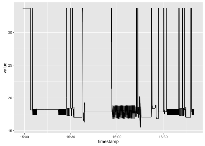
It looks like we have the position data items that we might need for this analysis in the log data. Let’s see the variation in position. We can plot all the data items in one plot using ggplot2.
Plotting the data
require("ggplot2")
## Loading required package: ggplot2
## Warning: package 'ggplot2' was built under R version 3.2.4
require("reshape2")
## Loading required package: reshape2
xpos_data = getDataItem(mtc_device, "Xposition") %>% getData()
ypos_data = getDataItem(mtc_device, "Yposition") %>% getData()
zpos_data = getDataItem(mtc_device, "Zposition") %>% getData()

ggplot() + geom_line(data = xpos_data, aes(x = timestamp, y = value))
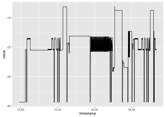
ggplot() + geom_line(data = ypos_data, aes(x = timestamp, y = value))
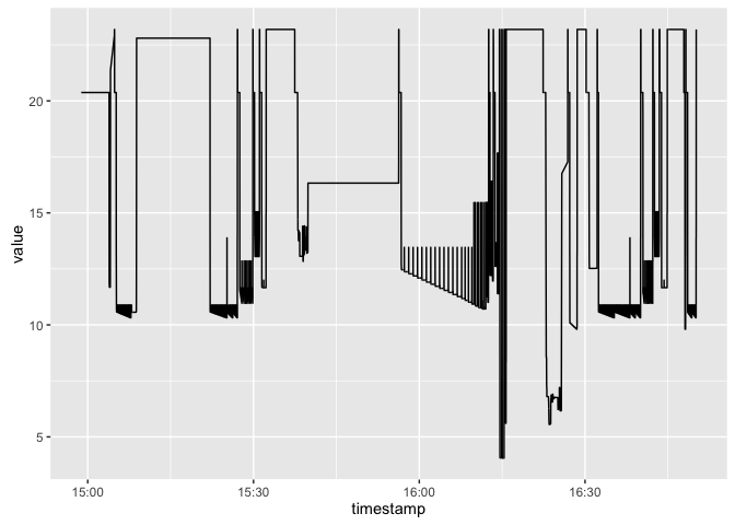
ggplot() + geom_line(data = zpos_data, aes(x = timestamp, y = value))
Merging different data items for simultaneous analysis
It looks like the machine is going back and forth quite some distance quite often, across
all the axes. We also don’t know how this traversal varies across different axis.
However, we can get a much better idea of the motion if we could plot one
axis against the other. For that we have to merge the different data items. Since the
different data items have different timestamp values as the key, it is not as straightforward
as doing a join of one data item against the other. For this purpose, the mtconnect packge has a merge
method defined for the MTCDevice Class
merged_pos_data = merge(mtc_device, "position") # merge all dataitems with the word position
head(merged_pos_data)
##                    timestamp
## 1 2015-11-02 14:58:49.994391
## 2 2015-11-02 14:59:03.742392
## 3 2015-11-02 14:59:03.886408
## 4 2015-11-02 14:59:14.122334
## 5 2015-11-02 14:59:14.270387
## 6 2015-11-02 14:59:22.486440
##   nist_testbed_GF_Agie_1<Device>:Aposition<ANGLE-ACTUAL>
## 1                                                -0.0001
## 2                                                -0.0001
## 3                                                -0.0001
## 4                                                -0.0001
## 5                                                -0.0001
## 6                                                -0.0001
##   nist_testbed_GF_Agie_1<Device>:Cposition<ANGLE-ACTUAL>
## 1                                                 0.0278
## 2                                                 0.0278
## 3                                                 0.0278
## 4                                                 0.0278
## 5                                                 0.0278
## 6                                                 0.0278
##   nist_testbed_GF_Agie_1<Device>:Xposition<POSITION-ACTUAL>
## 1                                                  33.69547
## 2                                                  33.69548
## 3                                                  33.69547
## 4                                                  33.69548
## 5                                                  33.69547
## 6                                                  33.69548
##   nist_testbed_GF_Agie_1<Device>:Yposition<POSITION-ACTUAL>
## 1                                                 -38.69783
## 2                                                 -38.69783
## 3                                                 -38.69783
## 4                                                 -38.69783
## 5                                                 -38.69783
## 6                                                 -38.69784
##   nist_testbed_GF_Agie_1<Device>:Zposition<POSITION-ACTUAL>
## 1                                                  20.37543
## 2                                                  20.37543
## 3                                                  20.37543
## 4                                                  20.37543
## 5                                                  20.37543
## 6                                                  20.37543
Oops. Looks like we have also merged in the angular position. Let’s try a more
directed merge. Also, the names of the data items have the full xpaths attached to them. While this might be
useful in other circumstances to get the hierarchical position of the data, we can dispense with it
now using the extract_param_from_xpath function. Let’s view the data after that
merged_pos_data = merge(mtc_device, "position<POSITION-ACTUAL") # merge all dataitems with the word position
names(merged_pos_data) = extract_param_from_xpath(names(merged_pos_data), param = "DIName", show_warnings = F)
head(merged_pos_data)
##                    timestamp Xposition Yposition Zposition
## 1 2015-11-02 14:58:49.994391  33.69547 -38.69783  20.37543
## 2 2015-11-02 14:59:03.742392  33.69548 -38.69783  20.37543
## 3 2015-11-02 14:59:03.886408  33.69547 -38.69783  20.37543
## 4 2015-11-02 14:59:14.122334  33.69548 -38.69783  20.37543
## 5 2015-11-02 14:59:14.270387  33.69547 -38.69783  20.37543
## 6 2015-11-02 14:59:22.486440  33.69548 -38.69784  20.37543
Much better. Now let’s plot the data items in one shot.
ggplot(data = merged_pos_data, aes(x = timestamp)) +
  geom_line(aes(y = Xposition, col = 'Xpos')) +
  geom_line(aes(y = Yposition, col = 'Ypos')) +
  geom_line(aes(y = Zposition, col = 'Zpos')) +
  theme(legend.title = element_blank())
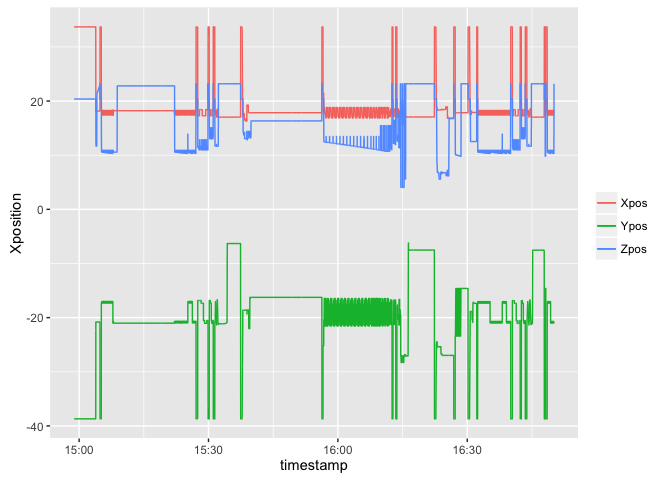
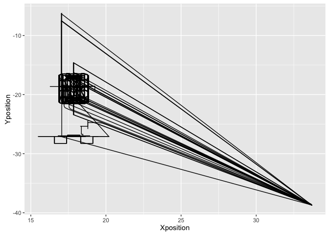
It does look the sudden traverals are simultaenous across the axes. Plotting one axes against the other leads to the same conclusion. It also gives us an idea of the different representations of the part
ggplot(data = merged_pos_data, aes(x = Xposition, y = Yposition)) + geom_path()

ggplot(data = merged_pos_data, aes(x = Xposition, y = Zposition)) + geom_path()
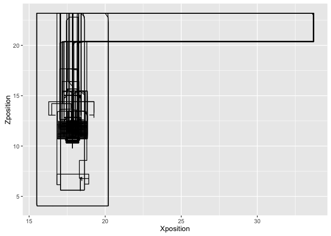
ggplot(data = merged_pos_data, aes(x = Zposition, y = Yposition)) + geom_path()
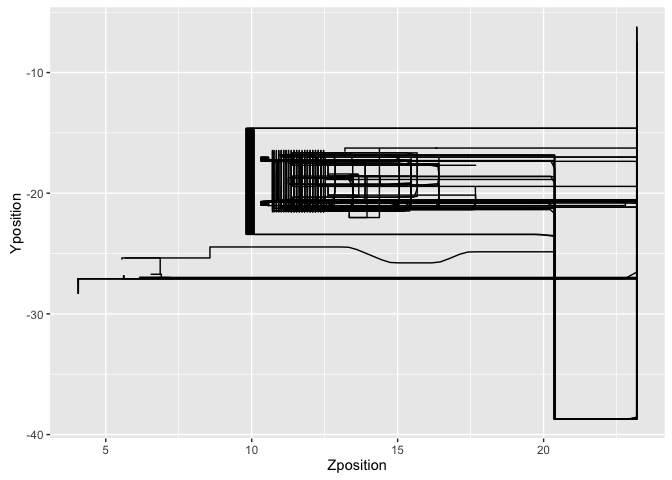
So the machine tool is going to the origin every so often.
Deriving new process parameters
It might help our analysis to also calculate a few process parameters that the machine tool is not providing directly. Here we are going to calculate the actual Path Feedrate of the machine as it executes the process using the position data.
Derived Path Feedrate
Path Feedrate can be calculated as the rate of change of the position values. Here, we must use the 3-dimensional distance value and not just one of the position vectors.
PFR = Total Distance / Total Time = Sqrt(Sum of Squares of distane along individual axis) / time taken for motion
position_change_3d =
((lead(merged_pos_data$Xposition, 1) - merged_pos_data$Xposition) ^ 2 +
(lead(merged_pos_data$Yposition, 1) - merged_pos_data$Yposition) ^ 2 +
(lead(merged_pos_data$Zposition, 1) - merged_pos_data$Zposition) ^ 2 ) ^ 0.5
merged_pos_data$time_taken =
lead(as.numeric(merged_pos_data$timestamp), 1) - as.numeric(merged_pos_data$timestamp)
merged_pos_data$pfr = round(position_change_3d / merged_pos_data$time_taken, 4)
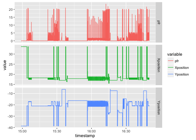
dt.df <- melt(merged_pos_data, measure.vars = c("pfr", "Xposition", "Yposition"))
ggplot(dt.df, aes(x = timestamp, y = value)) +
geom_line(aes(color = variable)) +
facet_grid(variable ~ ., scales = "free_y")
## Warning: Removed 1 rows containing missing values (geom_path).
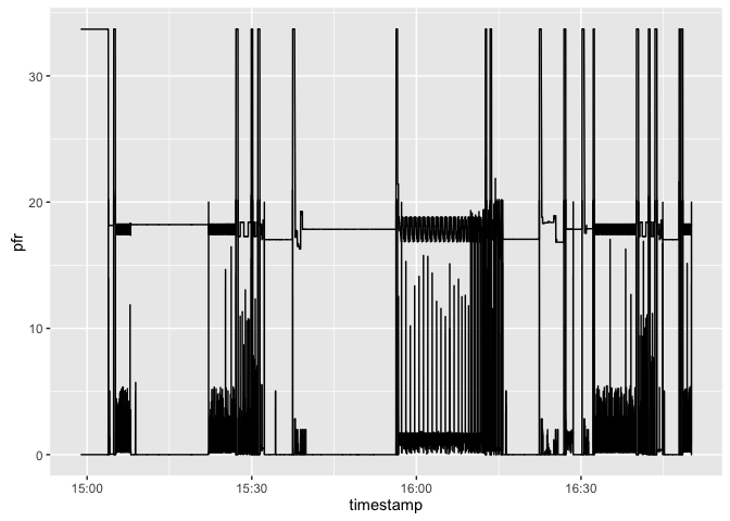
ggplot(data = merged_pos_data, aes(x = timestamp)) +
  geom_step(aes(y = pfr)) +
  geom_step(aes(y = Xposition))
## Warning: Removed 1 rows containing missing values (geom_path).
Let’s add this derived data back into the MTCDevice Class.
pfr_data = merged_pos_data %>% select(timestamp, value = pfr) # Structuring data correctly
mtc_device = add_data_item_to_mtc_device(mtc_device, pfr_data, data_item_name = "pfr<PATH_FEEDRATE>",
                                         data_item_type = "Sample", source_type = "calculated")
names(mtc_device@data_item_list)
##  [1] "nist_testbed_GF_Agie_1<Device>:Aposition<ANGLE-ACTUAL>"
##  [2] "nist_testbed_GF_Agie_1<Device>:avail<AVAILABILITY>"
##  [3] "nist_testbed_GF_Agie_1<Device>:Cposition<ANGLE-ACTUAL>"
##  [4] "nist_testbed_GF_Agie_1<Device>:estop<EMERGENCY_STOP>"
##  [5] "nist_testbed_GF_Agie_1<Device>:execution<EXECUTION>"
##  [6] "nist_testbed_GF_Agie_1<Device>:Fovr<PATH_FEEDRATE-OVERRIDE>"
##  [7] "nist_testbed_GF_Agie_1<Device>:line<LINE>"
##  [8] "nist_testbed_GF_Agie_1<Device>:logic<LOGIC_PROGRAM>:81000045___69 COOLANT SWITCHED OFF<CONDITION>"
##  [9] "nist_testbed_GF_Agie_1<Device>:logic<LOGIC_PROGRAM>:81000046___70 FEED OVERRIDE = 0 %<CONDITION>"
## [10] "nist_testbed_GF_Agie_1<Device>:mode<CONTROLLER_MODE>"
## [11] "nist_testbed_GF_Agie_1<Device>:move<x:MOTION>"
## [12] "nist_testbed_GF_Agie_1<Device>:program<PROGRAM>"
## [13] "nist_testbed_GF_Agie_1<Device>:Sovr<SPINDLE_SPEED-OVERRIDE>"
## [14] "nist_testbed_GF_Agie_1<Device>:system<SYSTEM>:34___Stylus already in contact<CONDITION>"
## [15] "nist_testbed_GF_Agie_1<Device>:system<SYSTEM>:36___Probe system not ready<CONDITION>"
## [16] "nist_testbed_GF_Agie_1<Device>:system<SYSTEM>:3AA___Key non-functional<CONDITION>"
## [17] "nist_testbed_GF_Agie_1<Device>:system<SYSTEM>:454A___Limit switch Y+<CONDITION>"
## [18] "nist_testbed_GF_Agie_1<Device>:Xposition<POSITION-ACTUAL>"
## [19] "nist_testbed_GF_Agie_1<Device>:Yposition<POSITION-ACTUAL>"
## [20] "nist_testbed_GF_Agie_1<Device>:Zposition<POSITION-ACTUAL>"
## [21] "pfr<PATH_FEEDRATE>"
Identifying Inefficiencies
Idle times
Our first task is to identify the periods when the machine was idle. For this we can use a few approaches.
- Find out the times when the execution status was not active OR
- Find out the times when the machine was not feeding (PFR~0) OR
- Find the periods when the feed override was zero
We will be trying out all the approaches and choosing union of the three as the period when machine is idle.
# Getting all the relevant data
merged_data = merge(mtc_device, "EXECUTION|PATH_FEEDRATE|POSITION")
names(merged_data) = extract_param_from_xpath(names(merged_data), param = "DIName", show_warnings = F)

merged_data = merged_data %>%
  mutate(exec_idle = F, feed_idle = F, override_idle = F) %>% # Setting everything false by default
  mutate(exec_idle = replace(exec_idle, !(execution %in% "ACTIVE"), TRUE)) %>%
  mutate(feed_idle = replace(feed_idle, pfr < 0.01, TRUE)) %>%
  mutate(override_idle = replace(override_idle, Fovr < 1, TRUE)) %>%
  mutate(machine_idle = as.logical(exec_idle + feed_idle + override_idle))
head(merged_data)
##                    timestamp execution   Fovr Xposition Yposition
## 1 2015-11-02 14:58:49.990541      <NA> 111.25        NA        NA
## 2 2015-11-02 14:58:49.994391      <NA> 111.25  33.69547 -38.69783
## 3 2015-11-02 14:59:03.742392      <NA> 111.25  33.69548 -38.69783
## 4 2015-11-02 14:59:03.886408      <NA> 111.25  33.69547 -38.69783
## 5 2015-11-02 14:59:14.122334      <NA> 111.25  33.69548 -38.69783
## 6 2015-11-02 14:59:14.270387      <NA> 111.25  33.69547 -38.69783
##   Zposition    pfr exec_idle feed_idle override_idle machine_idle
## 1        NA     NA      TRUE     FALSE         FALSE         TRUE
## 2  20.37543 0.0000      TRUE      TRUE         FALSE         TRUE
## 3  20.37543 0.0001      TRUE      TRUE         FALSE         TRUE
## 4  20.37543 0.0000      TRUE      TRUE         FALSE         TRUE
## 5  20.37543 0.0001      TRUE      TRUE         FALSE         TRUE
## 6  20.37543 0.0000      TRUE      TRUE         FALSE         TRUE
Machine tool at origin
We need to identify the time spent by the machine at origin. Let’s look at the X - Y graph again
ggplot(data = merged_pos_data, aes(x = Xposition, y = Yposition)) + geom_path()
It is clear that the periods when the machine was origin are roughly X > 30, Y < -30. Adding this into the mix
merged_data_final = merged_data %>%
  mutate(at_origin = F) %>% # Setting everything false by default
  mutate(at_origin = replace(at_origin, Xposition > 30 & Yposition < -30, TRUE)) %>%
  select(timestamp, machine_idle, at_origin)
head(merged_data_final)
##                    timestamp machine_idle at_origin
## 1 2015-11-02 14:58:49.990541         TRUE     FALSE
## 2 2015-11-02 14:58:49.994391         TRUE      TRUE
## 3 2015-11-02 14:59:03.742392         TRUE      TRUE
## 4 2015-11-02 14:59:03.886408         TRUE      TRUE
## 5 2015-11-02 14:59:14.122334         TRUE      TRUE
## 6 2015-11-02 14:59:14.270387         TRUE      TRUE
Calculating Summary Statistics
Now we have all the data at our disposal to calculate the time statistics. First we
need to convert the time series into interval format to get the duratins. We can use
convert_ts_to_interval function to do the same.
merged_data_intervals = convert_ts_to_interval(merged_data_final)
head(merged_data_intervals)
##                        start                        end duration
## 1 2015-11-02 14:58:49.990541 2015-11-02 08:58:49.994391     0.00
## 2 2015-11-02 14:58:49.994391 2015-11-02 08:59:03.742392    13.75
## 3 2015-11-02 14:59:03.742392 2015-11-02 08:59:03.886408     0.14
## 4 2015-11-02 14:59:03.886408 2015-11-02 08:59:14.122334    10.24
## 5 2015-11-02 14:59:14.122334 2015-11-02 08:59:14.270387     0.15
## 6 2015-11-02 14:59:14.270387 2015-11-02 08:59:22.486440     8.22
##   machine_idle at_origin
## 1         TRUE     FALSE
## 2         TRUE      TRUE
## 3         TRUE      TRUE
## 4         TRUE      TRUE
## 5         TRUE      TRUE
## 6         TRUE      TRUE
Now we can aggregate across the different states to find the total amount of time in each state.
time_summary = merged_data_intervals %>% group_by(machine_idle, at_origin) %>%
  summarise(total_time = sum(duration, na.rm = T))

print(time_summary)
## Source: local data frame [4 x 3]
## Groups: machine_idle [?]
##
##   machine_idle at_origin total_time
##          (lgl)     (lgl)      (dbl)
## 1        FALSE     FALSE    2713.77
## 2        FALSE      TRUE      21.99
## 3         TRUE     FALSE    3339.20
## 4         TRUE      TRUE     576.95
total_time = sum(time_summary$total_time)
efficient_time = sum(time_summary$total_time[1])
inefficient_time = sum(time_summary$total_time[2:4])
interrupted_time = sum(time_summary$total_time[3:4])
time_at_origin = sum(time_summary$total_time[c(2,4)])
## [1] "Results"
## [1] "Total Time of Operation (including interruptions) = 6651.91s"
## [1] "Total Time without identified inefficiencies = 2713.77s"
## [1] "Total Time wasted due to interruptions = 3916.15s"
## [1] "Total Time wasted due to being at origin = 598.94s"