
NOTE: This is a repost of an article that was first published in 2016, updated to for latest version
Introduction
Every so often while doing data analysis, I have come across a situation where I have two datasets, which have the same structure but with small differences in the actual data between the two. For example:
- Variation of a dataset across different time periods for the same grouping
- Variation of values for different algorithms, etc.
In the above cases, I want to easily identify what has changed across the two data.frames,
how much has changed, and also hopefully to get a quick summary of the extent of change. There are
packages like the compare package on R, which have focused more on the structure of
the data frame and lesser on the data itself. I was not able to easily identify and
isolate what has changed in the data itself. So I decided to write one for myself. That is
what compareDF package is all about.
The output can be visualized either on the RStudio Viewer, or sent to a file as an HTML or an XLSX file.
Installation
You can install the CRAN version of the package as below:
install.packages("compareDF")
Development version can be installed using devtools
devtools::install_github('alexsanjoseph/compareDF')
Usage
The package has a single function, compare_df. It takes in two data frames, and one or
more grouping variables and does a comparison between the the two. In addition you can
specify columns to ignore, decide how many rows of changes to be displayed in the case
of the HTML output, and decide what tolerance you want to provide to detect change.
Basic Example
Let’s take the example of a teacher who wants to compare the marks and grades of students across two years, 2010 and 2011. The data is stored in tabular format.
library(compareDF)
data("results_2010", "results_2011")
print(results_2010)
print(results_2011)
The data shows the performance of students in two divisions, A and B for two years. Some subjects like Maths, Physics, Chemistry and Art are given scores while others like Discipline and PE are given grades.
It is possible that there are students of the same name in two divisions, for example, there is a Rohit in both the divisions in 2011.
It is also possible that some students have dropped out, or added new across the two years. Eg: - Mugger and Dhakkan dropped out while Vikram and Dikchik where added in the Division B
The package allows a user to quickly identify these changes.
Basic Comparison
Now let’s compare the performance of the students across the years. The grouping variables are the Student column. We will ignore the Division column and assume that the student names are unique across divisions. In this sub-example, if a student appears in two divisions, he/she has studied in both of them.
ctable_student = compare_df(results_2011, results_2010, c("Student"))
ctable_student$comparison_df
By default, no columns are excluded from the comparison, so any of the tuple of grouping
variables which are different across the two data frames are shown in the comparison table.
The comparison_df table shows all the rows for which at least one record has changed. Conversely, if
nothing has changed across the two tables, the rows are not displayed. If a new record has been
introduced or a record has been removed, those are displayed as well.
For example, Akshay, Division A has had the exact same scores but has two different grades for Discipline across the two years so that row is included.
However, Macho, Division B has had the exact same scores in both the years for all subjects, so his data is not shown in the comparison table.
HTML Output
While the comparison table can be quickly summarized in various forms for futher analysis, it is
very difficult to process visually. The html_output provides a way to represent this is a way that is easier
for the numan eye to read. NOTE: You need to install the htmlTable package for the HTML comparison to work.
create_output_table(ctable_student)
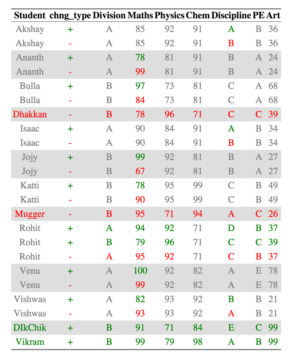
Now it is very easy to see recognize what has changed. A single cell is colored if it has changed across the two datasets. The value of the cell in the older dataset is colored red and the value of the cell in the newer dataset is colored green. Cells that haven’t changed across the two datasets are colored grey.
If a new row was introduced, the Row group names (and all the other columns for that row as well ) are colored in Green. Similarly, a row group name (and the other columns in that row) are colored red if a row was removed.
For Example, Akshay, Ananth and Bulla has had changes in scores, which are in Discipline, Maths, and Maths respectively. Dhakkan and Mugger have dropped out of the dataset from 2010 and the all the columns for the rows are shown in red, which DikChik and Vikram have joined new in the data set and all the columns for the rows are in green.
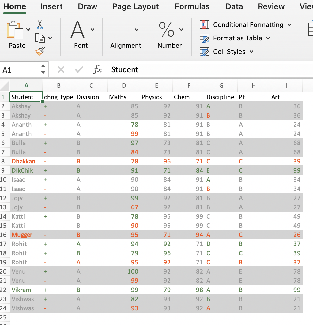
XLSX Output
Alternately you can write to an xlsx file as well
create_output_table(ctable_student, output_type = 'xlsx', file_name = "test_file.xlsx")
Change Count and Summary
You can get an details of what has changed for each group using
the change_count object in the output. A summary
of the same is provided in the change_summary object.
ctable_student$change_count
ctable_student$change_summary
Grouping Multiple Columns
We can also group_multiple columns into the grouping variable
ctable_student_div = compare_df(results_2011, results_2010, c("Division", "Student"))
ctable_student_div$comparison_df
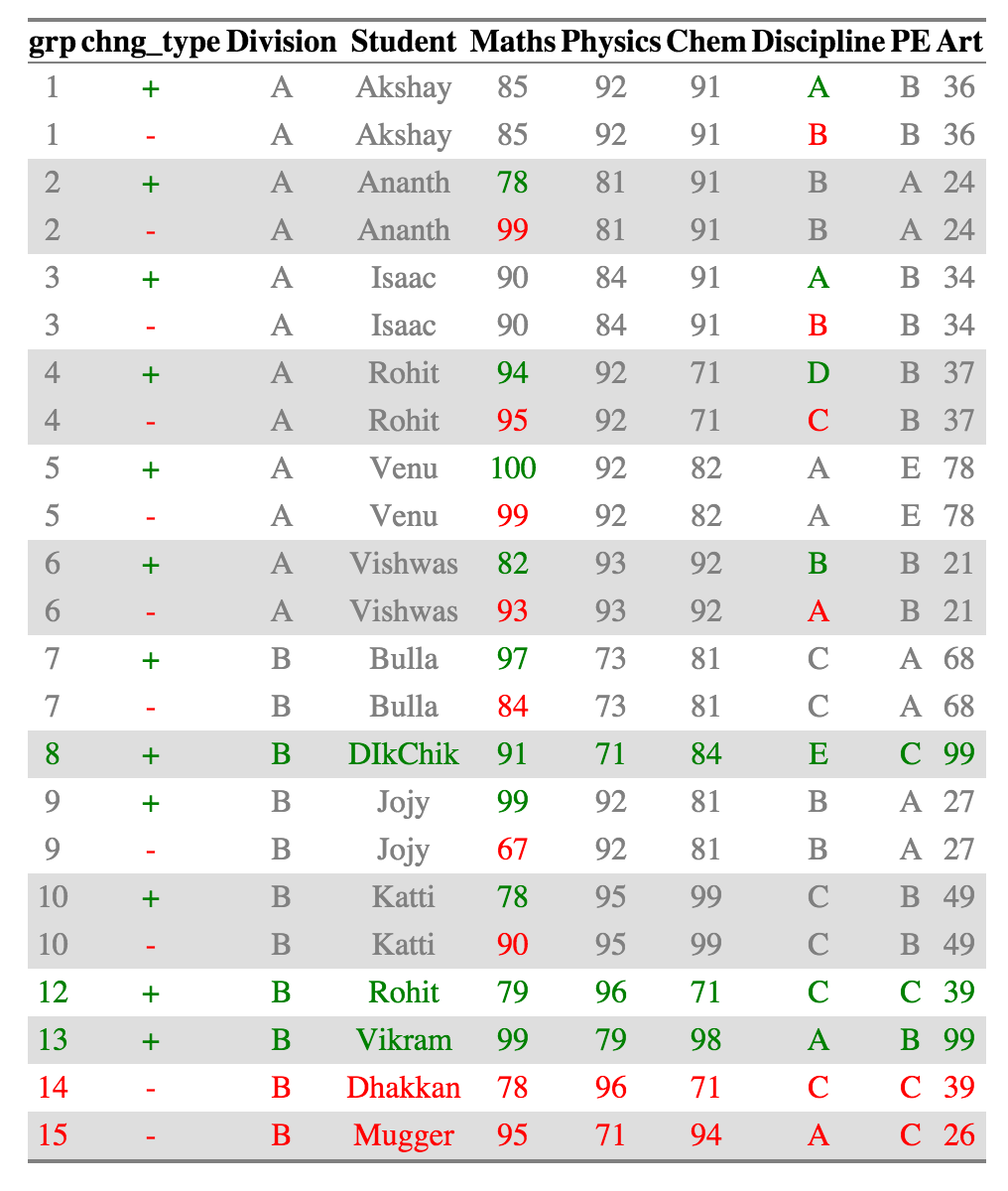
Now Rohits in each individual division are considered as belonging to separate groups and compared accordingly. All the other summaries also change appropriately.
Excluding certain Columns
You can ignore certain columns using the exclude parameter. The fields that have to be excluded can be given as a character vector. (This is a convenience function to deal with the case where some columns are not included)
Preserving all rows
The default behavior of the compare_df function is to show only the records that have changed. Sometimes the use might want to preserve all the records even after the comparison and not just see the values that have been changed (especially in the HTML). In this case, you can set the keep_unchanged parameter to TRUE.
Limiting HTML size
For dataframes which have a large amount of differences in them, generating HTML might take
a long time and crash your system. So the maximum diff size for the HTML (and for the HTML
visualization only) is capped at 100 by default. If you want to see more difference, you can change
the limit_html parameter appropriately. NOTE: This is only of the HTML output which is used for visual
checking. The main comparison data frame and the summaries ALWAYS include data from all the rows.
Changing color
You can use the color_scheme parameter to change the color of the cells generated. The parameter must me a named vector or a list with the appropriate names - The default values are c("addition" = "green", "removal" = "red", "unchanged_cell" = "gray", "unchanged_row" = "deepskyblue") but can be changed as needed by the user.
Tolerance
It is possible that you’d like numbers very close to each other to be ignored. For example,
if the marks of a student vary by less that 5% across the years, it could be due to random
error and not any real performance indictaor. In such a case, you would want to give a tolerance
parameter. For this case, giving a tolerance of 0.05 would ignore all the changes that are
less than 5% apart from the lower value.
ctable_student_div = compare_df(results_2011, results_2010, c("Division", "Student"), tolerance = 0.05)
create_output_table(ctable_student_div)
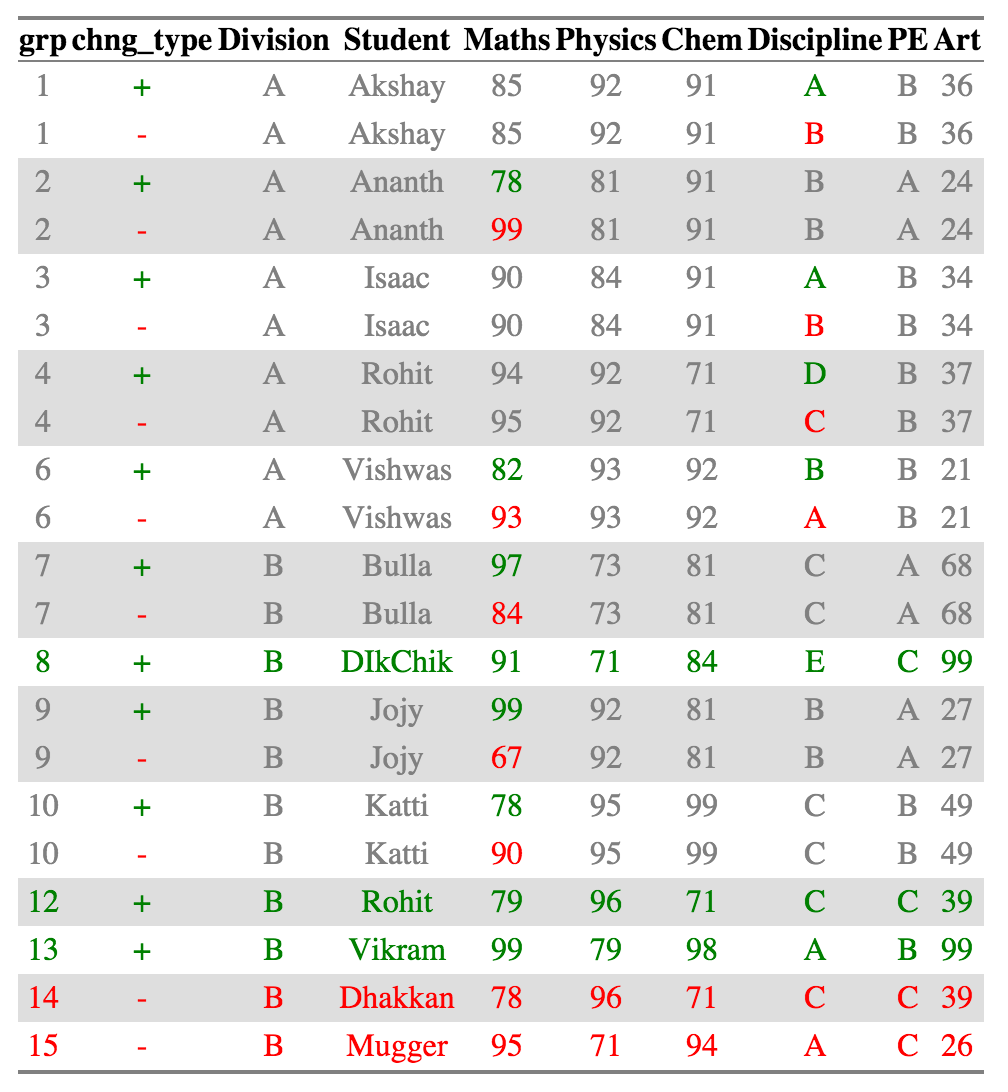
Venu from division A who had a score change from 100 to 99 is no longer present in the diff calculation or in the output
Naturally, tolerance has no meaning for non-numeric values.
Additional features
- set the color scheme in the output using the
color_schemeargument - preserve the rows that have not changed in the analysis using the
keep_unchanged_rowsargument - use
differenceas an argument to use difference rather than ratio for tolerance - options to name the columns in the output
- option change column name
- option to change group column name
- keep only the columns which have changed using
keep_unchanged_cols - convert output to wide format using
create_wide_output - customize nomenclature of the chng_type using
change_markers